
作者|Marcellus Ruben
编译|VK
来源|Towards Datas Science

当你听到“茶”和“咖啡”这个词时,你会怎么看这两个词?也许你会说它们都是饮料,含有一定量的咖啡因。关键是,我们可以很容易地认识到这两个词是相互关联的。然而,当我们把“tea”和“coffee”两个词提供给计算机时,它无法像我们一样识别这两个词之间的关联。
单词不是计算机自然就能理解的东西。为了让计算机理解单词背后的意思,这个单词需要被编码成数字形式。这就是词嵌入的用武之地。
词嵌入是自然语言处理中常用的一种技术,将单词转换成向量形式的数值。这些向量将以一定的维数占据嵌入空间。
如果两个词有相似的语境,比如“tea”和“coffee”,那么这两个词在嵌入空间中的距离将彼此接近,而与具有不同语境的其他词之间的距离则会更远。
在这篇文章中,我将逐步向你展示如何可视化嵌入这个词。由于本文的重点不是详细解释词嵌入背后的基本理论,你可以在本文和本文中阅读更多关于该理论的内容。
为了可视化词嵌入,我们将使用常见的降维技术,如PCA和t-SNE。为了将单词映射到嵌入空间中的向量表示,我们使用预训练词嵌入GloVe 。
加载预训练好的词嵌入模型
在可视化词嵌入之前,通常我们需要先训练模型。然而,词嵌入训练在计算上是非常昂贵的。因此,通常使用预训练好的词嵌入模型。它包含嵌入空间中的单词及其相关的向量表示。
GloVe是斯坦福大学研究人员在Google开发的word2vec之外开发的一种流行的预训练词嵌入模型。在本文中,实现了GloVe预训练的词嵌入,你可以在这里下载它。
https://nlp.stanford.edu/projects/glove/
同时,我们可以使用Gensim库来加载预训练好的词嵌入模型。可以使用pip命令安装库,如下所示。
pip install gensim作为第一步,我们需要将GloVe文件格式转换为word2vec文件格式。通过word2vec文件格式,我们可以使用Gensim库将预训练好的词嵌入模型加载到内存中。由于每次调用此命令时,加载此文件都需要一些时间,因此,如果仅为此目的而使用单独的Python文件,则会更好。
import pickle
from gensim.test.utils import datapath, get_tmpfile
from gensim.models import KeyedVectors
from gensim.scripts.glove2word2vec import glove2word2vec

glove_file = datapath('C:/Users/Desktop/glove.6B.100d.txt')
word2vec_glove_file = get_tmpfile("glove.6B.100d.word2vec.txt")
glove2word2vec(glove_file, word2vec_glove_file)

model = KeyedVectors.load_word2vec_format(word2vec_glove_file)

filename = 'glove2word2vec_model.sav'
pickle.dump(model, open(filename, 'wb'))
创建输入词并生成相似单词
现在我们有了一个Python文件来加载预训练的模型,接下来我们可以在另一个Python文件中调用它来根据输入词生成最相似的单词。输入词可以是任何词。
输入单词后,下一步就是创建一个代码来读取它。然后,我们需要根据模型生成的每个输入词指定相似单词的数量。最后,我们将相似单词的结果存储在一个列表中。下面是实现此目的的代码。
import pickle

filename = 'glove2word2vec_model.sav'
model = pickle.load(open(filename, 'rb'))

def append_list(sim_words, words):

    list_of_words = []

    for i in range(len(sim_words)):

        sim_words_list = list(sim_words[i])
        sim_words_list.append(words)
        sim_words_tuple = tuple(sim_words_list)
        list_of_words.append(sim_words_tuple)

    return list_of_words

input_word = 'school'
user_input = [x.strip() for x in input_word.split(',')]
result_word = []

for words in user_input:

        sim_words = model.most_similar(words, topn = 5)
        sim_words = append_list(sim_words, words)

        result_word.extend(sim_words)

similar_word = [word[0] for word in result_word]
similarity = [word[1] for word in result_word]
similar_word.extend(user_input)
labels = [word[2] for word in result_word]
label_dict = dict([(y,x+1) for x,y in enumerate(set(labels))])
color_map = [label_dict[x] for x in labels]举个例子,假设我们想找出与“school”相关联的5个最相似的单词。因此,“school”将是我们的输入词。我们的结果是‘college’, ‘schools’, ‘elementary’, ‘students’, 和‘student’。
基于PCA的可视化词嵌入
现在,我们已经有了输入词和基于它生成的相似词。下一步,是时候让我们把它们在嵌入空间中可视化了。
通过预训练的模型,每个单词都可以用向量表示映射到嵌入空间中。然而,词嵌入具有很高的维数,这意味着无法可视化单词。
通常采用主成分分析(PCA)等方法来降低词嵌入的维数。简言之,PCA是一种特征提取技术,它将变量组合起来,然后在保留变量中有价值的部分的同时去掉最不重要的变量。如果你想深入研究PCA,我推荐这篇文章。
https://towardsdatascience.com/a-one-stop-shop-for-principal-component-analysis-5582fb7e0a9c
有了PCA,我们可以在2D或3D中可视化词嵌入,因此,让我们创建代码,使用我们在上面代码块中调用的模型来可视化词嵌入。在下面的代码中,只显示三维可视化。为了在二维可视化主成分分析,只应用微小的改变。你可以在代码的注释部分找到需要更改的部分。
import plotly
import numpy as np
import plotly.graph_objs as go
from sklearn.decomposition import PCA
def display_pca_scatterplot_3D(model, user_input=None, words=None, label=None, color_map=None, topn=5, sample=10):
if words == None:
if sample > 0:
words = np.random.choice(list(model.vocab.keys()), sample)
else:
words = [ word for word in model.vocab ]
word_vectors = np.array([model[w] for w in words])
three_dim = PCA(random_state=0).fit_transform(word_vectors)[:,:3]
# 对于2D,将three_dim变量改为two_dim,如下所示:
# two_dim = PCA(random_state=0).fit_transform(word_vectors)[:,:2]
data = []
count = 0
for i in range (len(user_input)):
trace = go.Scatter3d(
x = three_dim[count:count+topn,0],
y = three_dim[count:count+topn,1],
z = three_dim[count:count+topn,2],
text = words[count:count+topn],
name = user_input[i],
textposition = "top center",
textfont_size = 20,
mode = 'markers+text',
marker = {
'size': 10,
'opacity': 0.8,
'color': 2
}
)
#对于2D,不是使用go.Scatter3d,我们需要用go.Scatter并删除变量z。另外,不要使用变量three_dim,而是使用前面声明的变量(例如two_dim)
data.append(trace)
count = count+topn
trace_input = go.Scatter3d(
x = three_dim[count:,0],
y = three_dim[count:,1],
z = three_dim[count:,2],
text = words[count:],
name = 'input words',
textposition = "top center",
textfont_size = 20,
mode = 'markers+text',
marker = {
'size': 10,
'opacity': 1,
'color': 'black'
}
)
# 对于2D,不是使用go.Scatter3d,我们需要用go.Scatter并删除变量z。另外,不要使用变量three_dim,而是使用前面声明的变量(例如two_dim)
data.append(trace_input)
# 配置布局
layout = go.Layout(
margin = {'l': 0, 'r': 0, 'b': 0, 't': 0},
showlegend=True,
legend=dict(
x=1,
y=0.5,
font=dict(
family="Courier New",
size=25,
color="black"
)),
font = dict(
family = " Courier New ",
size = 15),
autosize = False,
width = 1000,
height = 1000
)
plot_figure = go.Figure(data = data, layout = layout)
plot_figure.show()
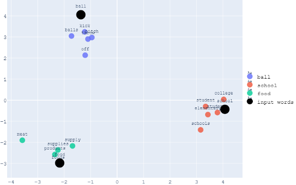
display_pca_scatterplot_3D(model, user_input, similar_word, labels, color_map)举个例子,让我们假设我们想把最相似的5个词与“ball”、“school”和“food”联系起来。下面是二维可视化的例子。
下面是同一组单词的三维可视化。
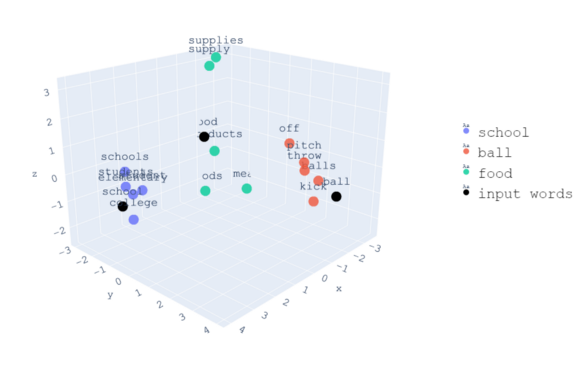
从视觉上,我们现在可以看到关于这些词所占空间的模式。与“ball”相关的单词彼此靠近,因为它们具有相似的上下文。同时,它们与“学校”和“食物”相关的词之间的距离因它们的语境不同而进一步不同。
基于t-SNE的可视化词嵌入
除了PCA,另一种常用的降维技术是t分布随机邻域嵌入(t-SNE)。PCA和t-SNE的区别是它们实现降维的基本技术。
PCA是一种线性降维方法。将高维空间中的数据线性映射到低维空间,同时使数据的方差最大化。同时,t-SNE是一种非线性降维方法。该算法利用t-SNE计算高维和低维空间的相似性。其次,利用一种优化方法,例如梯度下降法,最小化两个空间中的相似性差异。
用t-SNE实现词嵌入的可视化代码与PCA的代码非常相似。在下面的代码中,只显示三维可视化。为了使t-SNE在2D中可视化,只需应用微小的更改。你可以在代码的注释部分找到需要更改的部分。
import plotly
import numpy as np
import plotly.graph_objs as go
from sklearn.manifold import TSNE
def display_tsne_scatterplot_3D(model, user_input=None, words=None, label=None, color_map=None, perplexity = 0, learning_rate = 0, iteration = 0, topn=5, sample=10):
if words == None:
if sample > 0:
words = np.random.choice(list(model.vocab.keys()), sample)
else:
words = [ word for word in model.vocab ]
word_vectors = np.array([model[w] for w in words])
three_dim = TSNE(n_components = 3, random_state=0, perplexity = perplexity, learning_rate = learning_rate, n_iter = iteration).fit_transform(word_vectors)[:,:3]
# 对于2D,将three_dim变量改为two_dim,如下所示:
# two_dim = TSNE(n_components = 2, random_state=0, perplexity = perplexity, learning_rate = learning_rate, n_iter = iteration).fit_transform(word_vectors)[:,:2]
data = []
count = 0
for i in range (len(user_input)):
trace = go.Scatter3d(
x = three_dim[count:count+topn,0],
y = three_dim[count:count+topn,1],
z = three_dim[count:count+topn,2],
text = words[count:count+topn],
name = user_input[i],
textposition = "top center",
textfont_size = 20,
mode = 'markers+text',
marker = {
'size': 10,
'opacity': 0.8,
'color': 2
}
)
# 对于2D,不是使用go.Scatter3d,我们需要用go.Scatter并删除变量z。另外,不要使用变量three_dim,而是使用前面声明的变量(例如two_dim)
data.append(trace)
count = count+topn
trace_input = go.Scatter3d(
x = three_dim[count:,0],
y = three_dim[count:,1],
z = three_dim[count:,2],
text = words[count:],
name = 'input words',
textposition = "top center",
textfont_size = 20,
mode = 'markers+text',
marker = {
'size': 10,
'opacity': 1,
'color': 'black'
}
)
# 对于2D,不是使用go.Scatter3d,我们需要用go.Scatter并删除变量z。另外,不要使用变量three_dim,而是使用前面声明的变量(例如two_dim)
data.append(trace_input)
# 配置布局
layout = go.Layout(
margin = {'l': 0, 'r': 0, 'b': 0, 't': 0},
showlegend=True,
legend=dict(
x=1,
y=0.5,
font=dict(
family="Courier New",
size=25,
color="black"
)),
font = dict(
family = " Courier New ",
size = 15),
autosize = False,
width = 1000,
height = 1000
)
plot_figure = go.Figure(data = data, layout = layout)
plot_figure.show()
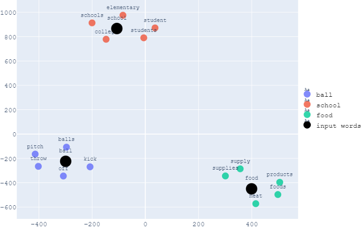
display_tsne_scatterplot_3D(model, user_input, similar_word, labels, color_map, 5, 500, 10000)与PCA可视化中相同的示例,即与“ball”、“school”和“food”相关的前5个最相似的单词的可视化结果如下所示。
下面是同一组单词的三维可视化。
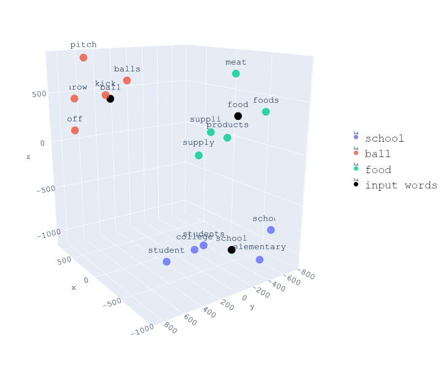
与PCA相同,注意具有相似上下文的单词彼此靠近,而具有不同上下文的单词则距离更远。
创建一个Web应用来可视化词嵌入
到目前为止,我们已经成功地创建了一个Python脚本,用PCA或t-SNE将词嵌入到2D或3D中。接下来,我们可以创建一个Python脚本来构建一个web应用程序,以获得更好的用户体验。
这个web应用程序使我们能够用大量的功能和交互性来可视化词嵌入。例如,用户可以键入自己的输入词,也可以选择与将返回的每个输入词相关联的前n个最相似的单词。
可以使用破折号或Streamlit创建web应用程序。在本文中,我将向你展示如何构建一个简单的交互式web应用程序,以可视化Streamlit的词嵌入。
首先,我们将使用之前创建的所有Python代码,并将它们放入一个Python脚本中。接下来,我们可以开始创建几个用户输入参数,如下所示:
-
降维技术,用户可以选择使用PCA还是t-SNE。因为只有两个选项,所以我们可以使用Streamlit中的selectbox属性。
-
可视化的维度,在这个维度中,用户可以选择将词嵌入2D还是3D显示。与之前一样,我们可以使用selectbox属性。
-
输入单词。这是一个用户输入参数,它要求用户键入他们想要的输入词,例如“ball”、“school”和“food”。因此,我们可以使用text_input属性。
-
Top-n最相似的单词,其中用户需要指定将返回的每个输入单词关联的相似单词的数量。因为我们可以选择任何数字。
接下来,我们需要考虑在我们决定使用t-SNE时会出现的参数。在t-SNE中,我们可以调整一些参数以获得最佳的可视化结果。这些参数是复杂度、学习率和优化迭代次数。因此,在每个情况下,让用户指定这些参数的最佳值是不存在的。
因为我们使用的是Scikit learn,所以我们可以参考文档来找出这些参数的默认值。perplexity 的默认值是30,但是我们可以在5到50之间调整该值。学习率的默认值是300,但是我们可以在10到1000之间调整该值。最后,迭代次数的默认值是1000,但我们可以将该值调整为250。我们可以使用slider属性来创建这些参数值。
import streamlit as st

dim_red = st.sidebar.selectbox(
 'Select dimension reduction method',
 ('PCA','TSNE'))
dimension = st.sidebar.selectbox(
     "Select the dimension of the visualization",
     ('2D', '3D'))
user_input = st.sidebar.text_input("Type the word that you want to investigate. You can type more than one word by separating one word with other with comma (,)",'')
top_n = st.sidebar.slider('Select the amount of words associated with the input words you want to visualize ',
    5, 100, (5))
annotation = st.sidebar.radio(
     "Enable or disable the annotation on the visualization",
     ('On', 'Off'))

if dim_red == 'TSNE':
    perplexity = st.sidebar.slider('Adjust the perplexity. The perplexity is related to the number of nearest neighbors that is used in other manifold learning algorithms. Larger datasets usually require a larger perplexity',
    5, 50, (30))

    learning_rate = st.sidebar.slider('Adjust the learning rate',
    10, 1000, (200))

    iteration = st.sidebar.slider('Adjust the number of iteration',
    250, 100000, (1000))
现在我们已经介绍了构建我们的web应用程序所需的所有部分。最后,我们可以把这些东西打包成一个完整的脚本,如下所示。
import plotly
import plotly.graph_objs as go
import numpy as np
import pickle
import streamlit as st
from sklearn.decomposition import PCA
from sklearn.manifold import TSNE
filename = 'glove2word2vec_model.sav'
model = pickle.load(open(filename, 'rb'))
def append_list(sim_words, words):
list_of_words = []
for i in range(len(sim_words)):
sim_words_list = list(sim_words[i])
sim_words_list.append(words)
sim_words_tuple = tuple(sim_words_list)
list_of_words.append(sim_words_tuple)
return list_of_words
def display_scatterplot_3D(model, user_input=None, words=None, label=None, color_map=None, annotation='On', dim_red = 'PCA', perplexity = 0, learning_rate = 0, iteration = 0, topn=0, sample=10):
if words == None:
if sample > 0:
words = np.random.choice(list(model.vocab.keys()), sample)
else:
words = [ word for word in model.vocab ]
word_vectors = np.array([model[w] for w in words])
if dim_red == 'PCA':
three_dim = PCA(random_state=0).fit_transform(word_vectors)[:,:3]
else:
three_dim = TSNE(n_components = 3, random_state=0, perplexity = perplexity, learning_rate = learning_rate, n_iter = iteration).fit_transform(word_vectors)[:,:3]
color = 'blue'
quiver = go.Cone(
x = [0,0,0],
y = [0,0,0],
z = [0,0,0],
u = [1.5,0,0],
v = [0,1.5,0],
w = [0,0,1.5],
anchor = "tail",
colorscale = [[0, color] , [1, color]],
showscale = False
)
data = [quiver]
count = 0
for i in range (len(user_input)):
trace = go.Scatter3d(
x = three_dim[count:count+topn,0],
y = three_dim[count:count+topn,1],
z = three_dim[count:count+topn,2],
text = words[count:count+topn] if annotation == 'On' else '',
name = user_input[i],
textposition = "top center",
textfont_size = 30,
mode = 'markers+text',
marker = {
'size': 10,
'opacity': 0.8,
'color': 2
}
)
data.append(trace)
count = count+topn
trace_input = go.Scatter3d(
x = three_dim[count:,0],
y = three_dim[count:,1],
z = three_dim[count:,2],
text = words[count:],
name = 'input words',
textposition = "top center",
textfont_size = 30,
mode = 'markers+text',
marker = {
'size': 10,
'opacity': 1,
'color': 'black'
}
)
data.append(trace_input)
# 配置布局
layout = go.Layout(
margin = {'l': 0, 'r': 0, 'b': 0, 't': 0},
showlegend=True,
legend=dict(
x=1,
y=0.5,
font=dict(
family="Courier New",
size=25,
color="black"
)),
font = dict(
family = " Courier New ",
size = 15),
autosize = False,
width = 1000,
height = 1000
)
plot_figure = go.Figure(data = data, layout = layout)
st.plotly_chart(plot_figure)
def horizontal_bar(word, similarity):
similarity = [ round(elem, 2) for elem in similarity ]
data = go.Bar(
x= similarity,
y= word,
orientation='h',
text = similarity,
marker_color= 4,
textposition='auto')
layout = go.Layout(
font = dict(size=20),
xaxis = dict(showticklabels=False, automargin=True),
yaxis = dict(showticklabels=True, automargin=True,autorange="reversed"),
margin = dict(t=20, b= 20, r=10)
)
plot_figure = go.Figure(data = data, layout = layout)
st.plotly_chart(plot_figure)
def display_scatterplot_2D(model, user_input=None, words=None, label=None, color_map=None, annotation='On', dim_red = 'PCA', perplexity = 0, learning_rate = 0, iteration = 0, topn=0, sample=10):
if words == None:
if sample > 0:
words = np.random.choice(list(model.vocab.keys()), sample)
else:
words = [ word for word in model.vocab ]
word_vectors = np.array([model[w] for w in words])
if dim_red == 'PCA':
two_dim = PCA(random_state=0).fit_transform(word_vectors)[:,:2]
else:
two_dim = TSNE(random_state=0, perplexity = perplexity, learning_rate = learning_rate, n_iter = iteration).fit_transform(word_vectors)[:,:2]
data = []
count = 0
for i in range (len(user_input)):
trace = go.Scatter(
x = two_dim[count:count+topn,0],
y = two_dim[count:count+topn,1],
text = words[count:count+topn] if annotation == 'On' else '',
name = user_input[i],
textposition = "top center",
textfont_size = 20,
mode = 'markers+text',
marker = {
'size': 15,
'opacity': 0.8,
'color': 2
}
)
data.append(trace)
count = count+topn
trace_input = go.Scatter(
x = two_dim[count:,0],
y = two_dim[count:,1],
text = words[count:],
name = 'input words',
textposition = "top center",
textfont_size = 20,
mode = 'markers+text',
marker = {
'size': 25,
'opacity': 1,
'color': 'black'
}
)
data.append(trace_input)
# 配置布局
layout = go.Layout(
margin = {'l': 0, 'r': 0, 'b': 0, 't': 0},
showlegend=True,
hoverlabel=dict(
bgcolor="white",
font_size=20,
font_family="Courier New"),
legend=dict(
x=1,
y=0.5,
font=dict(
family="Courier New",
size=25,
color="black"
)),
font = dict(
family = " Courier New ",
size = 15),
autosize = False,
width = 1000,
height = 1000
)
plot_figure = go.Figure(data = data, layout = layout)
st.plotly_chart(plot_figure)
dim_red = st.sidebar.selectbox(
'Select dimension reduction method',
('PCA','TSNE'))
dimension = st.sidebar.selectbox(
"Select the dimension of the visualization",
('2D', '3D'))
user_input = st.sidebar.text_input("Type the word that you want to investigate. You can type more than one word by separating one word with other with comma (,)",'')
top_n = st.sidebar.slider('Select the amount of words associated with the input words you want to visualize ',
5, 100, (5))
annotation = st.sidebar.radio(
"Enable or disable the annotation on the visualization",
('On', 'Off'))
if dim_red == 'TSNE':
perplexity = st.sidebar.slider('Adjust the perplexity. The perplexity is related to the number of nearest neighbors that is used in other manifold learning algorithms. Larger datasets usually require a larger perplexity',
5, 50, (30))
learning_rate = st.sidebar.slider('Adjust the learning rate',
10, 1000, (200))
iteration = st.sidebar.slider('Adjust the number of iteration',
250, 100000, (1000))
else:
perplexity = 0
learning_rate = 0
iteration = 0
if user_input == '':
similar_word = None
labels = None
color_map = None
else:
user_input = [x.strip() for x in user_input.split(',')]
result_word = []
for words in user_input:
sim_words = model.most_similar(words, topn = top_n)
sim_words = append_list(sim_words, words)
result_word.extend(sim_words)
similar_word = [word[0] for word in result_word]
similarity = [word[1] for word in result_word]
similar_word.extend(user_input)
labels = [word[2] for word in result_word]
label_dict = dict([(y,x+1) for x,y in enumerate(set(labels))])
color_map = [label_dict[x] for x in labels]
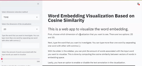
st.title('Word Embedding Visualization Based on Cosine Similarity')
st.header('This is a web app to visualize the word embedding.')
st.markdown('First, choose which dimension of visualization that you want to see. There are two options: 2D and 3D.')
st.markdown('Next, type the word that you want to investigate. You can type more than one word by separating one word with other with comma (,).')
st.markdown('With the slider in the sidebar, you can pick the amount of words associated with the input word you want to visualize. This is done by computing the cosine similarity between vectors of words in embedding space.')
st.markdown('Lastly, you have an option to enable or disable the text annotation in the visualization.')
if dimension == '2D':
st.header('2D Visualization')
st.write('For more detail about each point (just in case it is difficult to read the annotation), you can hover around each points to see the words. You can expand the visualization by clicking expand symbol in the top right corner of the visualization.')
display_pca_scatterplot_2D(model, user_input, similar_word, labels, color_map, annotation, dim_red, perplexity, learning_rate, iteration, top_n)
else:
st.header('3D Visualization')
st.write('For more detail about each point (just in case it is difficult to read the annotation), you can hover around each points to see the words. You can expand the visualization by clicking expand symbol in the top right corner of the visualization.')
display_pca_scatterplot_3D(model, user_input, similar_word, labels, color_map, annotation, dim_red, perplexity, learning_rate, iteration, top_n)
st.header('The Top 5 Most Similar Words for Each Input')
count=0
for i in range (len(user_input)):
st.write('The most similar words from '+str(user_input[i])+' are:')
horizontal_bar(similar_word[count:count+5], similarity[count:count+5])
count = count+top_n现在可以使用Conda提示符运行web应用程序。在提示符中,转到Python脚本的目录并键入以下命令:
$ streamlit run your_script_name.py接下来,会自动弹出一个浏览器窗口,你可以在这里本地访问你的web应用程序。下面是你可以使用该web应用程序执行的操作的快照。
就这样!你已经创建了一个简单的web应用程序,它具有很多交互性,可以用PCA或t-SNE可视化词嵌入。
如果你想看到这个词嵌入可视化的全部代码,你可以在我的GitHub页面上访问它。
https://github.com/marcellusruben/Word_Embedding_Visualization
原文链接:https://towardsdatascience.com/visualizing-word-embedding-with-pca-and-t-sne-961a692509f5
欢迎关注磐创AI博客站:
http://panchuang.net/
sklearn机器学习中文官方文档:
http://sklearn123.com/
欢迎关注磐创博客资源汇总站:
http://docs.panchuang.net/
原创文章,作者:磐石,如若转载,请注明出处:https://panchuang.net/2020/10/19/%e5%9f%ba%e4%ba%8epca%e5%92%8ct-sne%e5%8f%af%e8%a7%86%e5%8c%96%e8%af%8d%e5%b5%8c%e5%85%a5/
